Introduction to EECS
Deciding how to make trade-off is a crucial part of engineering. Programs should never be a mystery to you.
Overview
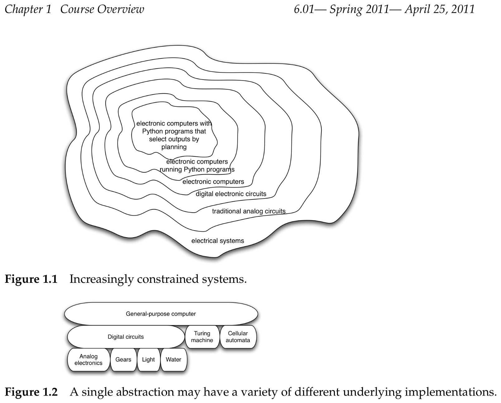
Modularity, abstraction and modeling
- Modularity is the idea of building components that can be re-used
- Abstraction is the idea that after constructing a module(be it software or circuits or gears)
-
The concept about
compilersorinterpretersThe languages are converted into instructions in the computer’s native machine language by other computer programs -
The one about the choice of programming language The choice of programming language is primarily a matter of taste and convenience
Models
It is a new system that is considerably simpler than system being modeled, but which captures the important aspects of the original system.
- Analytical models
- Synthetic models
- Internal models
- Data structures
Programs and Data
The object-oriented programming will give us methods fpr capturing common patterns in data and the procedures that operate on that data, via classes, generic functions, and inheritance.
The meaning of computer programs by understanding how the interpreter operates on them.
Interpreter
- Programs are understood and executed by a computer program called an interpreter
- The
readerortokenizertakes as input a string of characters and divides them intotokens, which are numbers, words(like while or a) and special characters(like :) - The
parsertakes as input the string of tokens and understands them as constructs in the programming language, such as while loops, procedure definitions, or return statements - The
evaluator(which is also sometimes called the interpreter, as well) has the really interesting job of determining the value and effects of the program that you ask it to interpret - The
printertakes the value returned by the evaluator and prints it out fo the user to see
3.1 Primitives
Primitive data(integers, floating point numbers, and strings)
Data structures(lists, arrays, dictionaries and records) in python language. Make DS allow us at the most basic level to think of a collection of primitive data elements.- Sometimes we want to think of a collection of data, like a set of objects, or a family tree, without worrying whether it is an array or a list in its basic representation.
Abstract data typesprovides a way of abstracting away from representational details and allowing us to focus on what the data really means.
3.3 Structured data
List mutation and shared structure
A tuple is a structure that is like a list, but it not mutable. String is a special kind of tuple.
Lambda constructor
lambda <var1>, ..., <varn> : <expr>
Recursive
- The base case
- Recursive case
8 Long-term decision-making and search
State-space search
- a(possibly infinite) set of
statesthe system can be in; - a
starting state, which is an element of the set of states; - a
goal test, which is a procedure that can be applied to any state, and returns True if that state can serve as a goal; - a
successorfunction, which takes a state and an action as input, and returns the new state that will result form taking the action in the state - a
legal action list, which is just a list of actions that can be legally executed in this domain
The basic structure
def search(initialState, goalTest, actions, successor):
    # goalTest with the starting state as parameters
    if goalTest(initialState):
        return [(None, initialState)]
    # a data structure handle the new node
    agenda =EmptyAgenda()
    add(SearchNode(None, initialState, None), agenda)
    while agenda!=[]:
        parent=getElement(agenda)
        # Pruning Rule 2: If there are multiple actions that lead from a state r to a state s, consider only one of them.
        newChildStates=[]
        for a in actions(parent.state):
            newS=successor(parent.state, a)
            newN=SearchNode(a, newS, parent)
            if goalTest(newS):
                return newN.path()
            # Pruning Rule 2
            elif newS in newChildStates:
                pass
            # Do not consider any path that visits the same state twice
            elif parent.inPath(newS):
                pass
            else:
                # Pruning Rule 2
                newChildStates.append(newS)
                add(newN, agenda)
    return None
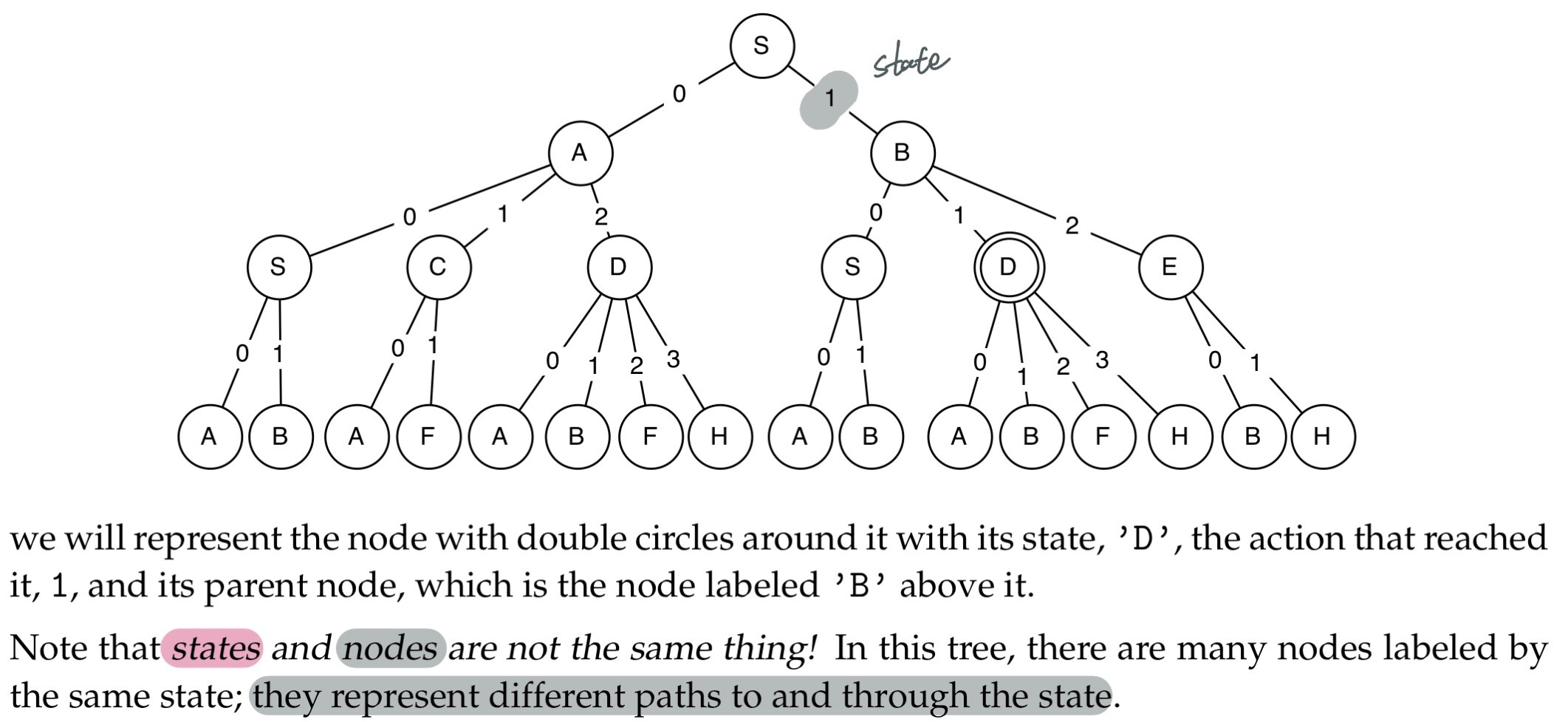
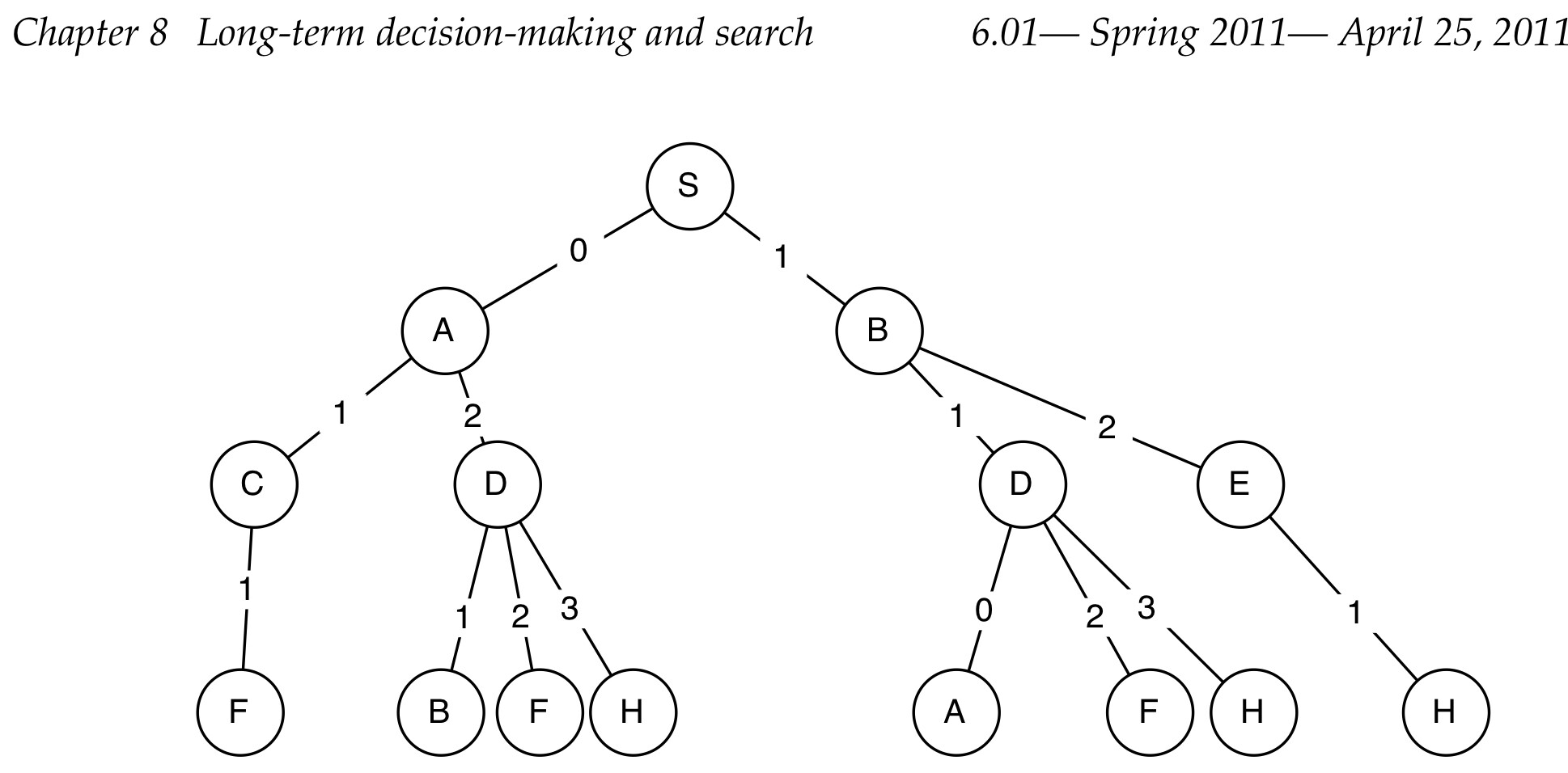
Representing search trees
We will start by defining a class to represent a search node
- the
stateof the node - the
actionthat was taken to arrive at the node - the search node from which this node can be reached(
parent)
class SearchNode:
    def __init__(self, action, state, parent):
        self.state=state
        self.action=action
        self.parent=parent
There are a couple of useful methods
- the
pathmethod, returns a list of pairs (a, s) corresponding to the path staring at the top(root) of the tree. It works its way up the tree, until it reaches a node whose parent is None
  def path(self):
      if self.parent==None:
        return [(self.action, self.states)]
      else:
        return self.parent.path() + [(self.action, self.state)]
- the
inPathmethod, which takes a state and returns True if the state occurs anywhere in the path from the root to the node
  def inPath(self, s):
      if s==self.state:
          return True
      elif self.parent==None:
          return False
      else:
          return self.parent.inPath(s)
Basic search algorithm
There are two plausible strategies:
- Start down a path, keep trying to extend it until you get stuck, in which case, go back to the last choice you had, and go a different way. This is how kids often solve mazes. We will call it
depth-firstsearch. - Go layer by layer through the tree, first considering all paths of length 1, than all the length 2, etc. We will call this
breadth-firstsearch.
There are some pruning rules:
- Do not consider any path that visits the same state twice(This can help to avoid trivial infinite loops)
- If there are multiple actions that lead from a state r to a state s, consider only one of them
- Do not consider any path that visits a state that you have already visited via some other path
Stacks and queues
In designing algorithms, we frequently make use of two simple data structures: stacks and queues. You can think of them both as abstract data types that support two operations: push and pop.
- stack: A stack is also called a LIFO, for
lastin,firstout - queue: A queue is also called a FIFO, for
firstin,firstout
In Python, we can use lists to represent both stacks and queues. If data is a list, then data.pop(0) removes the first element from the list and return it, and data.pop() removes the latest element and returns it.
Class Stack:
    def __init__(self):
        self.data=[]
    def push(self, item):
        self.data.append(item)
    def pop(self):
        return self.data.pop()
    def isEmpty(self):
        return self.data is []
Class Queue:
    def __init__(self):
        self.data=[]
    def push(self, item):
        self.data.append(item)
    def pop(self):
        return self.data.pop(0)
    def isEmpty(self):
        return self.data is []
Some important properties of depth-first-search:
- It will run forever if we do not apply pruning rule 1
- It may run forever in an infinite domain
- It does not necessarily find the shortest path
- It is generally efficient in the amount of space it requires to store the agenda, which will be a constant factor times the depth of the path it is currently considering
Some important properties od breadth-first search:
- Always returns a shortest(least number of steps) path to a goal state, if a goal state exists in the set of states reachable from the start state
- It may run forever if there is no solution and the domain is infinite
- It requires more space than depth-first search
def depthFirstSearch(initialState, goalTest, actions, successor)
    agenda=Stack()
    if goalTest(initialState)
        return [(None, initialState)]
    agenda.push(SearchNode(None, initialState, None))
    visited ={initialState: True}
    while not agenda.isEmpty():
        parent=agenda.pop()
        for a in actions(parent.state):
            newS=successor(parent.state, a)
            newN=SearchNode(a, newS, parent)
            if goalTest(newS):
                return newN.path()
            elif visited.has_key(newS):
                pass
            else:
                visited[newS]=True
                agenda.push(newN)
    return None
Computational complexity
The worst-case analysis for the algorithms
Let’s establish a bit of notation:
- b be the branching factor of the graph
- d be the maximum depth of thr graph
- l be the solution depth of the problem
- n be the state space size of the graph
Depth-first search, in the worst case, will search the entire search tree. The amount of storage it needs for the agenda is only b.d
Breadth-first search, only needs to search as deep as the depth of the best solution. So, breadth-first require visiting as many as b**steps nodes(worst situation)
Priority Queue
It is a data structure with the same basic operations as stacks and queues, with two difference:
- Items are pushed into priority queue with a numeric score, called a cost
- When it is time to pop an item, the item in the priority queue with the least code is returned and removed from the priority queue
Uniform-cost search algorithm
- It replace agenda with priority queue
- Instead of testing for a goal state when we put an element into the agenda, as we did in breadth-first search, we test for a goal state when we take an element out of the agenda. This crucial, to ensure that we actually find the shortest path to a goal state.